
EXPERIMENTAL DOSSIER
Wireless power transfer
From inductive coupling to a resonant setup: model, experiments, and documented results.
In this document
01 · Engineering question#
How does resonant tuning affect the efficiency and usable range of inductive power transfer? The preparatory-class bench connects an electrical model to real losses and geometry.
02 · Objectives#
- Compare non-resonant RL and resonant RLC operation.
- Explore frequency, coil separation, and misalignment.
- Observe voltages and energy transfer, then compare observations with the model.
03 · System architecture#
- Generator & excitation
- Transmitter RLC circuit
- Magnetic coupling
- Receiver RLC circuit
- Load
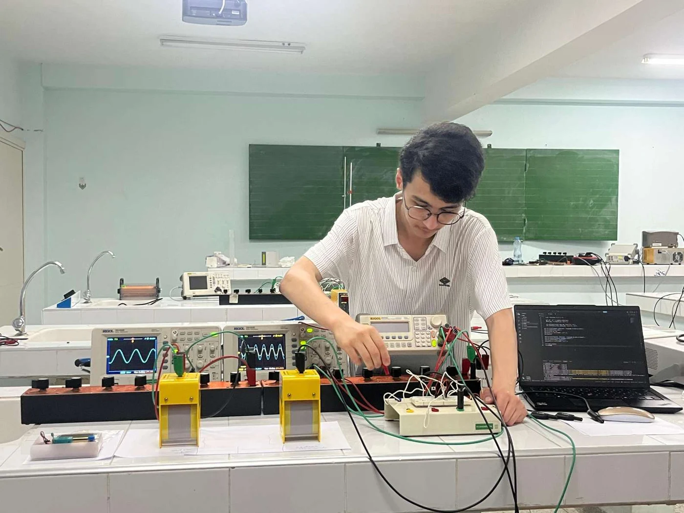
04 · Model & assumptions#
η = Poutput / Pinput
The LC relation locates resonance in an ideal circuit. Transfer between two coils also depends on mutual inductance, resistance, and load. Frequency alone therefore does not predict efficiency.
Note: resonance and tolerances05 · Engineering decisions#
Moving from RL to RLC allows comparison of resonant tuning. A frequency sweep identifies the operating region around 34 kHz; separation and alignment experiments then probe transfer robustness.
Coil dimensions and exact components must be taken from the original slides to reproduce the bench; substitute components are not presented here as equivalent.
06 · Experimental setup#
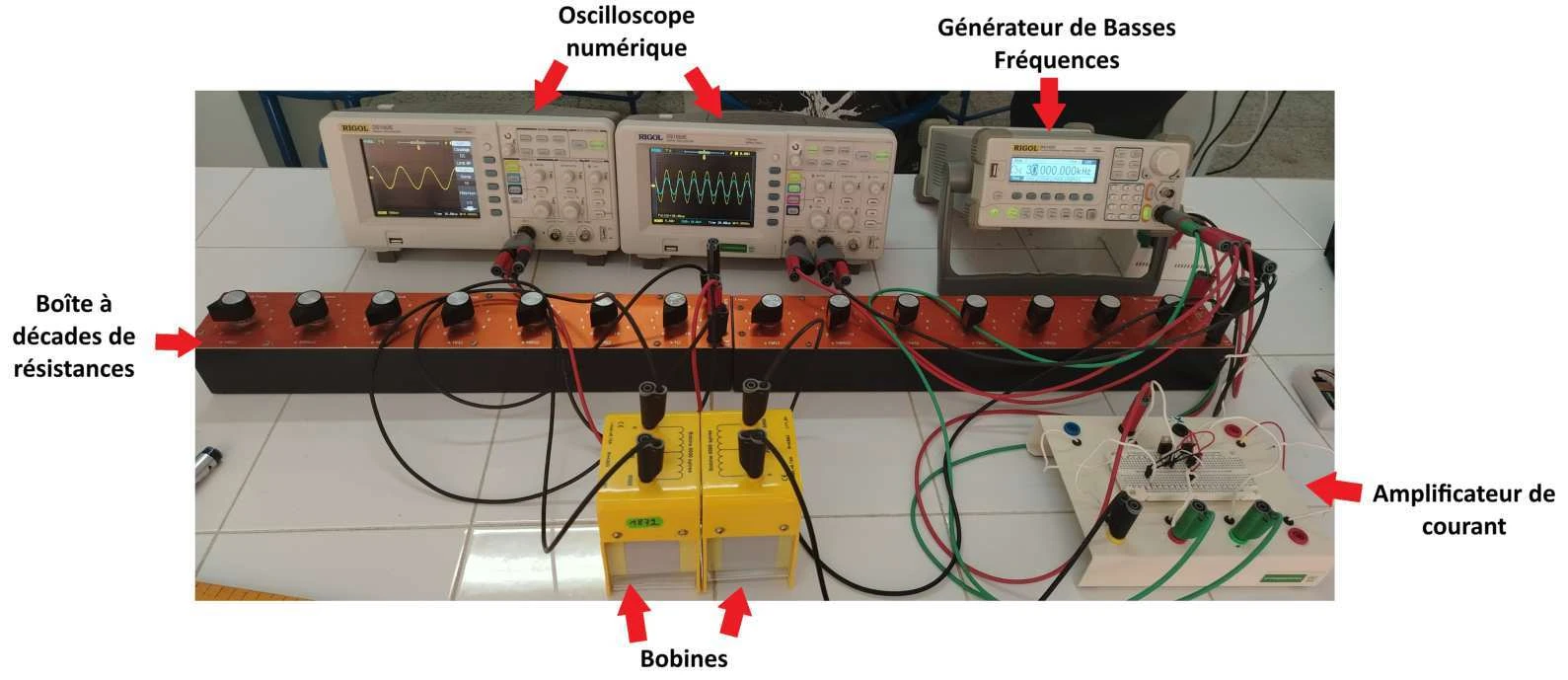
Equipment: digital oscilloscope, function generator, teaching coils, decade resistance box, and load components. Explored variables: frequency, axial separation, radial misalignment, and angle.
For a repeat experiment, record load, excitation, geometry, power calculation method, and instrument settings for each series. The downloadable log is blank.
07 · Results#
| Configuration | Reported peak efficiency | Frequency |
|---|---|---|
| Non-resonant coupling (RL) | 7.4% | Not specified for this peak |
| Resonant coupling (RLC) | 23% | 34 kHz |
These values compare the peaks of two configurations, not two measurements guaranteed to share the same frequency.
Source: TIPE presentation, slide 23The difference between the peaks is 15.6 percentage points. It describes this bench and these configurations; it is not a general performance claim for inductive transfer.
08 · Model and experiment#
The original slides compare theoretical and experimental curves. The reported resonant peak is at 34 kHz. A theoretical frequency calculated from measured L and C, together with traceable uncertainty, is needed before publishing a Δf discrepancy.
Parasitic resistance, geometry, component tolerances, and coupling are interpretation avenues. The interactive LC laboratory illustrates only the ideal model.
Explore the ideal model09 · Limitations#
- Results are specific to the tested configuration and load.
- No raw sweep dataset or complete uncertainty budget is included in this archive.
- Summary values come from the slides; they do not reconstruct a time series.
10 · Possible improvements#
- Characterize coils and losses with a traceable protocol.
- Automate sweeps and record raw measurements.
- Propagate uncertainty and compare several loads.
11 · Artifacts & references#
The slides are the project’s primary source. The log below is a retrospective summary, not a new laboratory measurement.
[1] Original presentation · 44 slidesEXP-001 · Peak comparisonBlank measurement template · CSV